We live in a world of dramatic change. Companies and societies are trying to tackle increasingly complex issues, and they are turning their attention to quantum technologies. Although it is expected to take some time before we see full-fledged quantum computers that utilize quantum phenomena, Toshiba is already working on quantum-inspired optimization technologies. We are applying our own in-house combinatorial optimization technologies for producing optimal results from massive numbers of options, providing them in the form of the quantum-inspired “SQBM+” optimization solution. This solution uses existing computers to produce highly accurate approximate solutions in short amounts of time. In this running feature, we will explain quantum-inspired optimization technologies.

In Part 1, we explained two methods in quantum computers and the positioning and structure of the quantum-inspired optimization technologies for them. In Part 2, we will explain bifurcation, which is an important element of these technologies, along with how processing is accelerated and improved, and we will provide an overview of the technologies.

In Part 1, we explained that the SQBM+ quantum-inspired optimization solution performed simulations of classicalized quantum bifurcation machines -- quantum computers that Toshiba is researching on its own. Simulations (numerical calculations) have been confirmed to produce high quality solutions to combinatorial optimization problems. The reason for this is not yet clear, but we believe that the idea of bifurcation is at work behind this algorithm.

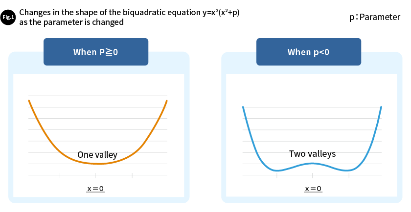
Bifurcation is a phenomenon in which a system’s state suddenly and dramatically changes in an instant, like when the number of cars on a road exceeds a certain number and a traffic jam suddenly occurs. When simulation (numerical calculation) or the like is used to make constant changes to something, the way the simulation proceeds may suddenly undergo a qualitative change. This is also referred to as bifurcation. Let’s explain using the biquadratic function y= x²(x²+p), which was used in a paper on a Simulated Bifurcation Algorithm (hereinafter “SB Algorithm”) published in 2019 (https://www.science.org/doi/10.1126/sciadv.aav2372). Here, “p” is a parameter. When parameter p is continuously changed, the simulation results also continuously change. With the SB Algorithm, parameter p is changed and the bifurcation phenomenon that occurs during the simulation (numerical calculation) is leveraged to achieve highly accurate combinatorial optimization.

Let’s look at this “y= x²(x²+p)” biquadratic equation.

• If we differentiate the biquadratic equation y= x²(x²+p), we get y'=2x(2x²+p).
• If we search for the x that produces y'=0 in order to find the extreme values of the equation, then setting 2x(2x²+p)=0, we can determine the following.
  (1) When p≧0, there is one extreme value: x=0
  (2) When p<0, there are three extreme values: x=0 and one value to each side of it

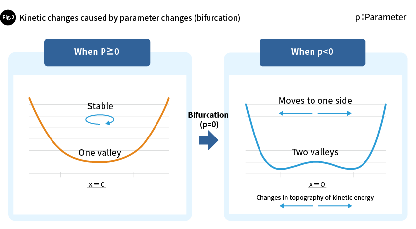
So for the biquadratic equation y=x²(x²+p), when p≧0, there is a single valley, at x=0. When p<0, there is a peak at x=0 and two valleys to either side of it (Fig. 1).

Hamiltonian equation in the SB Algorithm includes the aforementioned y=x²(x²+p) biquadratic equation in the portion that is equivalent to the kinetic energy of the Hamiltonian function that expresses the energy of a system. In accordance with this Hamiltonian equation, the SB Algorithm calculates the movement trajectory of a particle that is flying around erratically yet shaped by the contour lines (graph shape) of the kinetic energy defined by the biquadratic equation.

Let’s use the SB Algorithm to perform numerical calculation, gradually changing the value of parameter p from, for example, 1 to -1 (we will simplify the process of changing the parameter for this example). During this numerical calculation process, when p reaches zero, the biquadratic equation’s kinetic energy topography will suddenly switch from having one valley to having two. A particle which, until this point, was stably moving in the valley, around x=0, will suddenly become unstable. The particle will approach one of the two valleys that have newly appeared to the left and right of the origin, x=0, and will fall into the valley (Fig. 2).

With Ising machines like SQBM+, when performing combinatorial optimization problems like pathfinding problems, a function with a specific format is associated and the solution is determined by resolving the function to a minimization problem. With the SB Algorithm, a biquadratic equation is added to the function associated with the combinatorial optimization problem to cause further bifurcation, the contour lines of the combined kinetic energy are set, a particle moving irregularly along these contour lines is envisioned, and its trajectory is calculated.

Depending on the type of problem, there can be many input variables for the minimization function. For example, in the case of a pathfinding problem, numerous locations to be visited, and the distances between each, must be expressed. Based on the concepts of Hamiltonian mechanics, when SQBM+ is used to solve a combinatorial optimization, the way the two input variables of position and momentum are linked is that, for example, if there is a problem with 2,000 input variables, the trajectory of a particle moving in a 4,000-dimensional space is calculated.

SQBM+ gradually changes parameter p in this multidimensional space and performs numerical calculations as it does so. Bifurcation occurs in order, starting with the variable in the “position” dimension for which minimization has the greatest effect. As this numerical calculation proceeds, bifurcation occurs sequentially, determining if the variable that corresponds to “position” in each dimension is positive or negative. These positive and negative values are slightly changed to perform bifurcation in all dimensions. Finally, these “position” coordinate is read to determine the combinatorial optimization solution.

It appears that the successive bifurcation in each dimension is related to the SB Algorithm’s ability to produce good solutions to combinatorial optimization problems.

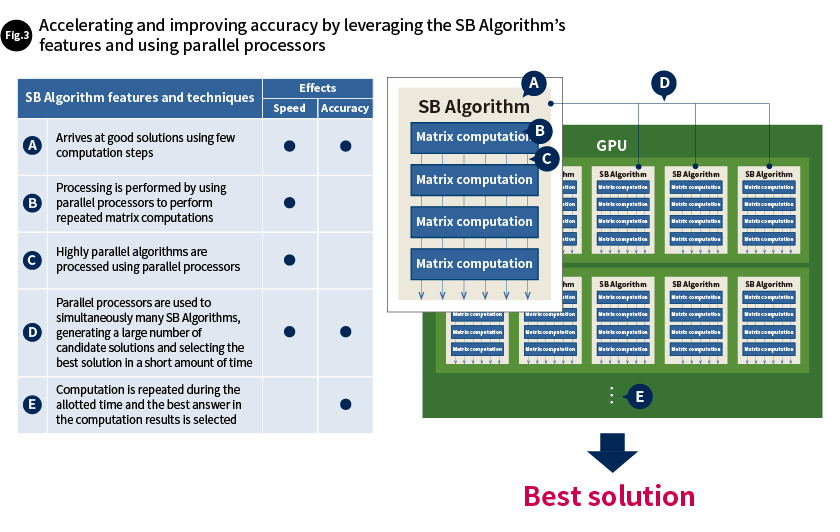
In Part 1, we explained how each of the SB Algorithm’s computation steps are extremely simple, how time-consuming matrix computations within each step can all be performed simultaneously, and how the system is highly matrix-oriented overall, providing good answers in short amounts of time. SQBM+ uses these features of the SB Algorithm while implementing them in a Graphics Processing Unit (GPU), taking advantage of the GPU’s ability to perform matrix computations such as image magnification, reduction, rotation, horizontal movement, and the like quickly and in parallel. The result is faster speeds and a higher level of accuracy.

The computation that takes the longest amount of time with the SB Algorithm is the matrix computation in each step. This is because matrix computation requires information for the position variable in every dimension. GPUs excel at this kind of matrix computation. SQBM+, which uses GPUs, can therefore rapidly perform matrix computation. For computation other than matrix computation, due to the nature of the SB Algorithm, which is highly parallel, calculations for each dimension can be performed independently. This means that SQBM+ can complete overall calculations extremely quickly.

Furthermore, not only does SQBM+ effectively leverage the features of GPUs, which excel at matrix computation, to rapidly perform SB Algorithm computation, but it also fully utilizes the tremendous computation resources of GPUs to run multiple SB Algorithms in parallel, improving accuracy. Depending on user settings, this parallel processing can be repeated multiple times so that it can get a better solution, further increasing the solution’s accuracy.

Unlike simulated annealing (SA), which uses a probabilistic algorithm, the SB Algorithm is a deterministic algorithm, so there are no probabilistic operations after initial values are decided, and the same routes are followed. In other words, if the same initial values are set, the solutions will always be identical. To make it possible to determine the best solution out of multiple solutions, given the characteristics of the SB Algorithm, SQBM+ runs multiple SB Algorithms in parallel repeatedly, only performing probabilistic operations when deciding initial values. Initial values are randomly assigned to produce diverse solutions. SQBM+ simulates the statistical production of various states by repeatedly performing parallel processing, increasing the accuracy of solutions. (Fig. 3)

To this point, we have explained the algorithm presented in a paper published in 2019. The algorithm presented in the paper is what we now call an adiabatic Simulated Bifurcation (aSB) algorithm. We further improved the algorithm in the process of practical use of services that take advantage of aSB algorithms. These improved algorithms are the ballistic Simulated Bifurcation (bSB) algorithm and the discrete Simulated Bifurcation (dSB) algorithm. SQBM+ services currently being provided by Azure Quantum, etc., use these two algorithms.

bSB uses the simple quadratic equation y=px² instead of the biquadratic equation y=x²(x²+p) to produce bifurcation (p is a parameter). For example, when the value of p is changed from 1 to -1 for this biquadratic equation, the origin changes from a valley to a peak (Fig. 4). If this function is used to draw kinetic energy landscapes, particles which were initially stably moving near the origin will fall away from the bifurcation border value of p=0 when p is changed.

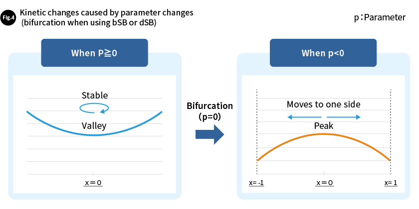
To prevent particles from rolling infinitely far away, walls were created at x=-1 or x=1 for bSB, and particles are restricted to the area between the two walls. bSB uses the bifurcation produced by a quadratic equation together with walls to perform numerical calculation by successively performing bifurcation from dimensions where minimization within the multidimensional space produces the greatest results, in the same way as with aSB. dSB uses the same quadratic equation as bSB, but to make it better suited to solving combinatorial optimization problems, the discrete nature of this type of problem is taken into consideration when choosing the direction of motion of the particles.

SQBM+ achieves a higher level of performance by using these new algorithms. This has been discussed in a paper published in 2021 (https://www.science.org/doi/10.1126/sciadv.abe7953).

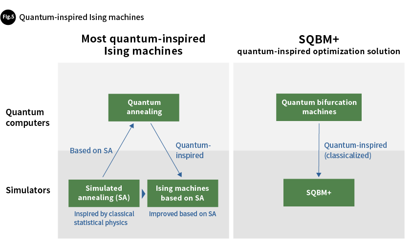
SQBM+ is the product of Toshiba’s own “quantum bifurcation machine” quantum computer, so it is a “quantum-inspired” Ising machine simulator (hereinafter an “Ising simulator”). Many of the Ising simulators currently on the market were inspired by quantum annealing, in which the principles of quantum mechanics are used to perform combinatorial optimization, so they are called “quantum-inspired.” Quantum annealing was invented in the 1990s as an extension of simulated annealing (SA), an optimization methodology developed in the 1980s that uses the classical physics field of statistical physics. Many quantum-inspired Ising simulators are based on simulated annealing. SQBM+’s origin point is the quantum bifurcation machine, which works with quanta from the very start, so it can be characterized as “native quantum-inspired.” (Fig. 5)

SQBM+ begins with equations that classicalize quantum bifurcation machines, but in the initial aSB stage, the already-classicalized equations were significantly reviewed and revised. When making further improvements, even more dramatic changes were made to the equations, producing the more advanced bSB and dSB algorithms. These improvements made it possible for SQBM+ to separate itself from the world of physical quantum hardware and explore concepts freely in the world of formulas. In the framework of the Hamiltonian equations of the classical world, which correspond to the Schrödinger’s equation of the quantum world, SQBM+ pursues even higher levels of performance based on unfettered software, mathematics, and physics concepts. We believe this is the key strength of SQBM+.

In Part 1, we explained the structure of the quantum-inspired optimization technologies that play important roles in SQBM+, which is centered on Ising machines. In Part 2, we have examined bifurcation in Simulated Bifurcation Algorithms and gotten an overview of quantum-inspired optimization technologies. In Part 3, we will be focusing on optimization. What is it? How are combinatorial optimization problems solved? We will answer these and other questions in detail, using concrete examples.

• Quantum-inspired Optimization Solutions “SQBM+”